In this assignment, I joined variables in tabular files to spatial maps files for Census Tracts (CTs) in both Metro Vancouver and Montréal. I then visualized and worked with rental housing cost data by exploring various methods for classifying quantitative data (monthly cost of rent) for Metro Vancouver CTs, comparing the monthly costs to Montréal, and also looked at another rental indicator which is housing affordability (the percent of people spending more than 30% of their income on rent).
Adapted the technique of ‘tabular join (of dbf files) to spatial layer files’ and various methods for classifying quantitative data for displaying rental cost (of housing) data in both Metro Vancouver and Montréal in 2016
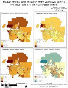
Natural breaks (Jenks) classify the data based on their distribution – the best method to fit the distribution of the map – it is more to be heterogeneous as the data is more likely to be evenly distributed according to different colors on a gradient as shown in the classification method. Equal Intervals classify the data based on classes with an equal range of values. However, this could result in an abundance of CTs with lower classes (classes at lower color ramp/gradient) as the classes at lower color ramp have a larger interval than the natural breaks method. There is a larger proportion/percentage of CTs falling in classes at lower color gradient than natural breaks due to higher class range (or higher individual class interval) – hence more values fall into classes at a lower color gradient. Manual Breaks require a change of break points/values manually by assigning different break values to the classes (in this case there is a range of around 500 equally for different classes). Standard deviation is rather a totally different method as it takes into account of diverging color scheme rather than sequential scheme as it takes into account of average, and higher and lower than average standard deviations – CTs with values lower than average are assigned with one sequence of color and higher than average assigned with another color sequence – this results in a similar spatial pattern with other method but is rather difficult for map users to understand due to incomprehensible classification method in term of using standard deviation rather than actual standardized data values.
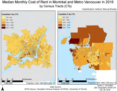
The data is collected from 2016 Census, Canadian Census Analyser (CHASS) as the rental costs need to be gathered for both Metro Vancouver and Montréal (2016 census from CHASS provides a complete list of the rental cost data) – there are a number of areas with no data values (no data available) as many CTs are not rental but owner dwellings such as in Kitsilano and Oakridge in Vancouver - this leads to error and uncertainty issues using this variable of monthly rental cost as it provides an incomplete list of monthly rental costs by CTs - data suppression (confidentially) issue - the specified population size for all areas or aggregations of standard areas is 40. Consequently, no characteristics or tabulated data are to be released for areas below a population size of 40. Absence of data variable averages for areas with respondents under 40 can be problematic in terms of areas with no rental cost data available - hence, the problem of drawing the non-visible boundaries arise as these are ‘conceptual’ boundaries that have been drawn based on the size of populations and hence it could also be problematic in constructing the boundaries for census administrative areas - should use housing/dwelling costs as the variable instead as the data is more to be complete
There are also other errors and uncertainty issues related as it is related to the MAUP - there are more variations of census data when aggregated over DAs than CTs – allowing more variations means more spatial accuracy of data. On the other hand, CTs are much less detailed Census data is aggregated over a larger census administrative area (CTs in this case). All the population in that administrative area is generalized to a mean, median, average value. E.g. Although statistics Canada tries to allocate areas based upon similar numbers of people, this allocation results in visual problems such as Stanley Park, the northernmost census tracks in North Vancouver and West Vancouver that are mostly forest (MAUP). Hence, there is an error with census mapping MAUP. Hence, MAUP could be regarded as a downside with creating CTs due to over-generalization of census data – however, creating DAs would be an advantage in this case due to more variations and accuracy of spatial data. The presence of only a few households with higher rental costs in a larger-sized CT can significantly impact the overall rental cost in the CT – e.g. the presence of outliers being taken into account can affect the overall mean and medians values of rental costs.
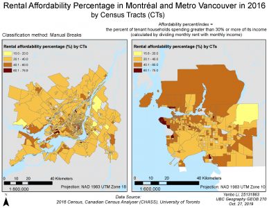
Affordability percent/index = the percent of tenant households spending greater than 30% or more of its income
It is a better indicator as rental cost alone would not be effective in terms of showing costs of living in a city as the (combined) household income might be sufficiently high to support high monthly rental cost – taking (monthly) household income into account for the rental cost and hence affordability would be more comprehensible than rental cost alone as it amounts the capacity or ability of an individual household to afford rental cost through combined income. Affordability could be regarded a good indicator of a city’s livability as tenant households who spend greater than 30% or more of its monthly (combined) income on rental cost would be classified as unaffordability due to a high amount of income used for paying off rental cost leaving lower disposable income – 30% or more on housing rents represents a higher burden for households.